| 编辑推荐: |
| 本文来源个人博客,本文将要讨论关于预测的方法。有一种预测是跟时间相关的,而这种处理与时间相关数据的方法叫做时间序列模型。 |
|
加载数据,观察数据
| %matplotlib
inline
import pandas as pd
import numpy as np
import matplotlib.pyplot as plt
import datetime
from dateutil.relativedelta import relativedelta
import seaborn as sns
import statsmodels.api as sm
from statsmodels.tsa.stattools import acf
from statsmodels.tsa.stattools import pacf
from statsmodels.tsa.seasonal import seasonal_decompose
df = pd.read_csv('portland-oregon-average-monthly.csv',
parse_dates=['month'], index_col='month')
print(df.head())
df['riders'].plot(figsize=(12,8), title= 'Monthly
Ridership', fontsize=14)
plt.savefig('month_ridership.png', bbox_inches='tight') |

分解数据:
decomposition = seasonal_decompose(df['riders'],
freq=12)
fig = plt.figure()
fig = decomposition.plot()
fig.set_size_inches(12, 6) |

时间序列稳定化
测试方法:
| from
statsmodels.tsa.stattools import adfuller
def test_stationarity(timeseries):
#Determing rolling statistics
rolmean = timeseries.rolling(window=12).mean()
rolstd = timeseries.rolling(window=12).std()
#Plot rolling statistics:
fig = plt.figure(figsize=(12, 8))
orig = plt.plot(timeseries, color='blue',label='Original')
mean = plt.plot(rolmean, color='red', label='Rolling
Mean')
std = plt.plot(rolstd, color='black', label
= 'Rolling Std')
plt.legend(loc='best')
plt.title('Rolling Mean & Standard Deviation')
plt.show()
#Perform Dickey-Fuller test:
print('Results of Dickey-Fuller Test:')
dftest = adfuller(timeseries, autolag='AIC')
dfoutput = pd.Series(dftest[0:4], index=['Test
Statistic','p-value','#Lags Used','Number of
Observations Used'])
for key,value in dftest[4].items():
dfoutput['Critical Value (%s)'%key] = value
print(dfoutput) |
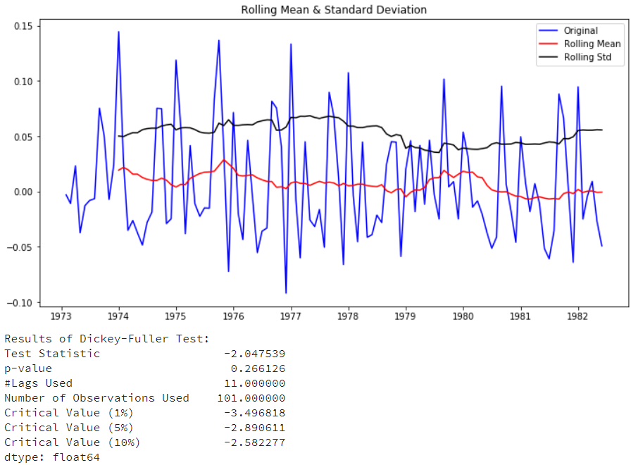
测试序列稳定性:
|
test_stationarity(df['riders']) |
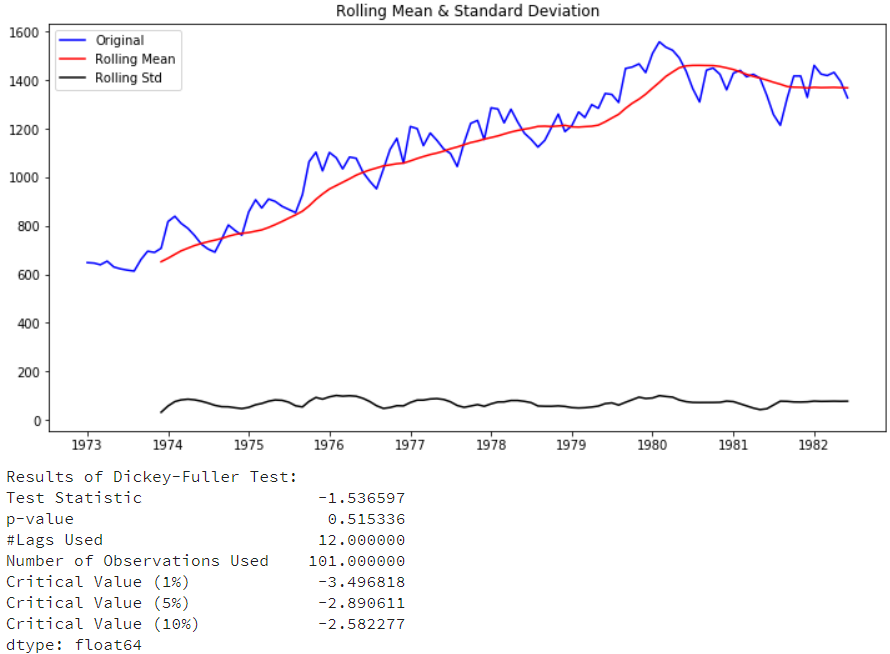
看以看到整体的序列并没有到达稳定性要求,要将时间序列转为平稳序列,有如下几种方法:
Deflation by CPI
Logarithmic(取对数)
First Difference(一阶差分)
Seasonal Difference(季节差分)
Seasonal Adjustment
这里会尝试取对数、一阶查分、季节差分三种方法,先进行一阶差分,去除增长趋势后检测稳定性:
| df['first_difference']
= df['riders'].
diff(1)
test_stationarity(df['first_difference'].
dropna(inplace=False)) |
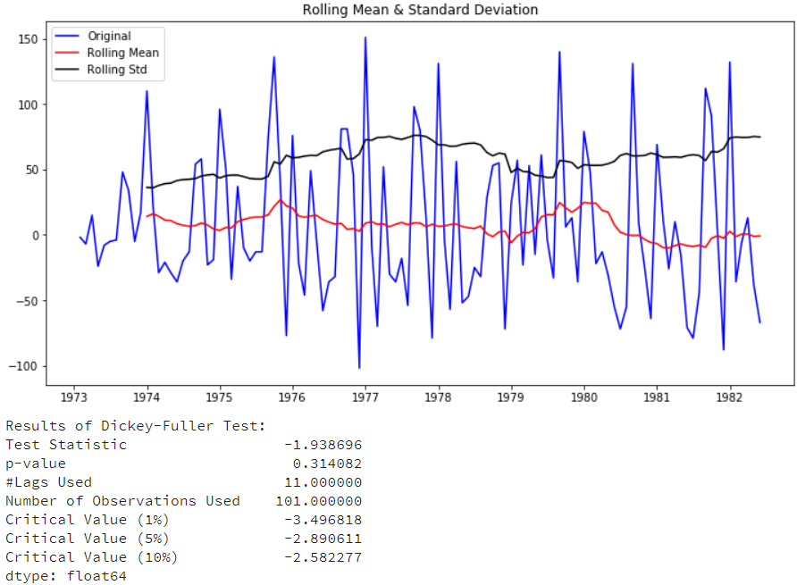
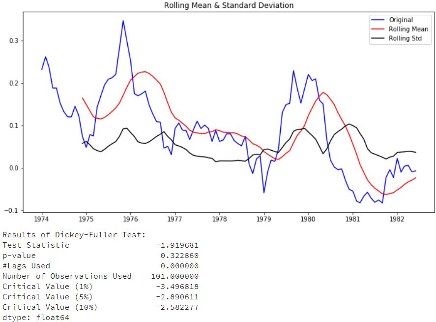
可以看到图形上看上去变稳定了,但p-value的并没有小于0.05。再来看看12阶查分(即季节查分),看看是否稳定:
| df['seasonal_difference']
= df
['riders'].diff(12)
test_stationarity(df['seasonal
_difference'].dropna(inplace=False))
|
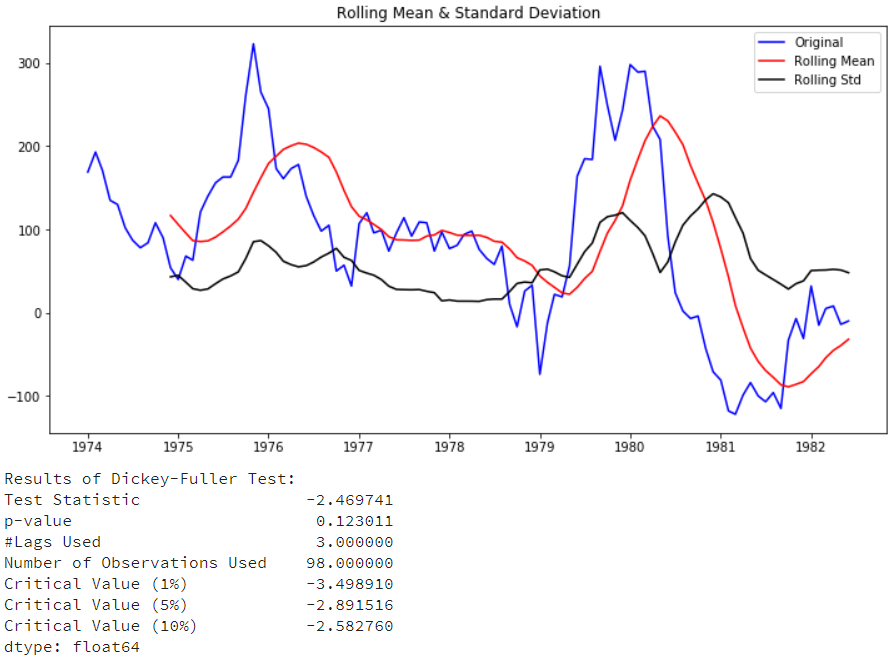
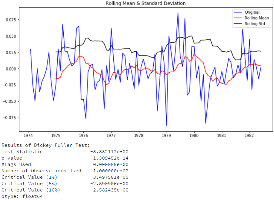
从图形上,比一阶差分更不稳定(虽然季节指标已经出来了),我们再来将一阶查分和季节查分合并起来,再来看下:
| df['seasonal_first_difference']
= df
['first_difference'].diff(12)
test_stationarity(df['seasonal_first
_difference'].dropna(inplace=False)) |

可以看到,在一阶差分后再加上季节差分,数据终于稳定下了。P-value小于了0.05,并且Test
Statistic的值远远小于Critical Value (5%)的值。
在《Analysis of Financial Time Series》提到,对原始数据取对数有两个用处:第一个是将指数增长转为线性增长;第二可以平稳序列的方差。再来看看取对数的数据:
|
df['riders_log']= np.log(df['riders'])
test_stationarity(df['riders_log']) |
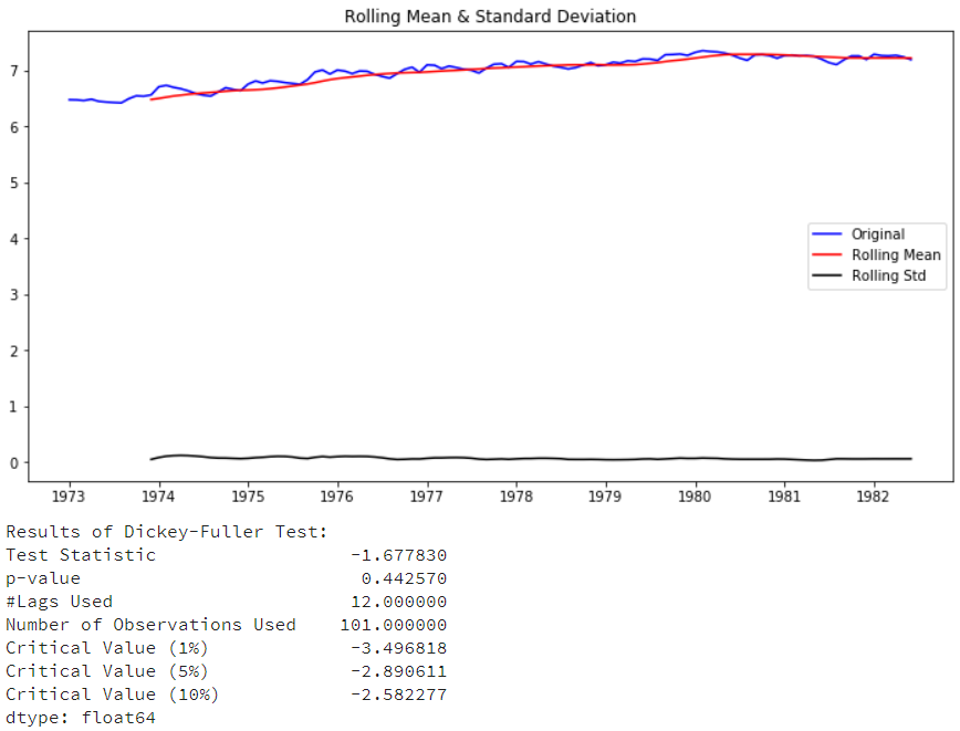
取对数后,从图形上看有些稳定了,但p-value还是没有接近0.05,没能达稳定性要求。在此基础上我们再来做下一阶差分,去除增长趋势:
| df['log_first_difference']
= df
['riders_log'].diff(1)
test_stationarity(df['log_first
_difference'].dropna(inplace=False)) |
还是没能满足需求,我们再来对对数进行季节性差分:
| df['log_seasonal_difference']
= df
['riders_log'].diff(12)
test_stationarity(df['log_seasonal
_difference'].dropna(inplace=False)) |
还是没能满足需求,再来试试在对数基础上进行一阶差分+季节差分的效果:
| df['log_seasonal_first_difference']
=
df['log_first_difference'].diff(12)
test_stationarity(df['log_seasonal_first
_difference'].dropna(inplace=False)) |
可以看到稳定了满足需求了,但是稳定性相比不取对数的情况下,并没有提升而是下降了。
绘制ACF和PACF图,找出最佳参数
| fig
= plt.figure(figsize=(12,8))
ax1 = fig.add_subplot(211)
fig = sm.graphics.tsa.plot_acf(df['seasonal
_first_difference'].iloc[13:],
lags=40, ax=ax1)
#从13开始是因为做季节性差分时window是12
ax2 = fig.add_subplot(212)
fig = sm.graphics.tsa.plot_pacf(df['seasonal_
first_difference'].iloc[13:],
lags=40, ax=ax2) |

fig = sm.graphics.tsa.plot_acf (
df [' seasonal _ first _ difference ' ] . iloc [ 13
: ], lags = 40 , ax = ax1 ) #从13开始是因为做季节性差分时window是12
一直搞不清楚这2张图怎么看。今天一起来学习下:(貌似下面的内容也是糊里糊涂的,后续还需更深入的学习)
如何确定差分阶数和常数项:
1.假如时间序列在很高的lag(10以上)上有正的ACF,则需要很高阶的差分
2.假如lag-1的ACF是0或负数或者非常小,则不需要很高的差分,假如lag-1的ACF是-0.5或更小,序列可能overdifferenced。
3.最优的差分阶数一般在最优阶数下标准差最小(但并不是总数如此)
4.模型不查分意味着原先序列是平稳的;1阶差分意味着原先序列有个固定的平均趋势;二阶差分意味着原先序列有个随时间变化的趋势
5.模型没有差分一般都有常数项;有两阶差分一般没常数项;假如1阶差分模型非零的平均趋势,则有常数项
如何确定AR和MA的阶数:
1.假如PACF显示截尾或者lag-1的ACF是正的(此时序列仍然有点underdifferenced),则需要考虑AR项;PACF的截尾项表明AR的阶数
2.假如ACF显示截尾或者lag-1的ACF是负的(此时序列有点overdifferenced),则需要加MA项,ACF的截尾项表明AR的阶数
3.AR和MA可以相互抵消对方的影响,所以假如用AR-MA模型去拟合数据,仍然需要考虑加些AR或MA项。尤其在原先模型需要超过10次的迭代去converge。
假如在AR部分有个单位根(AR系数和大约为1),此时应该减少一项AR增加一次差分
假如在MA部分有个单位根(MA系数和大约为1),此时应该减少一项AR减少一次差分
假如长期预测出现不稳定,则可能AR、MA系数有单位根
如何确定季节性部分:
1.假如序列有显著是季节性模式,则需要用季节性差分,但是不要使用两次季节性差分或总过超过两次差分(季节性和非季节性)
2.假如差分序列在滞后s处有正的ACF,s是季节的长度,则需要加入SAR项;假如差分序列在滞后s处有负的ACF,则需要加入SMA项,如果使用了季节性差异,则后一种情况很可能发生,如果数据具有稳定和合乎逻辑的季节性模式。如果没有使用季节性差异,前者很可能会发生,只有当季节性模式不稳定时才适用。应该尽量避免在同一模型中使用多于一个或两个季节性参数(SAR
+ SMA),因为这可能导致过度拟合数据和/或估算中的问题。
创建模型并进行预测
经过上面的分析,可以独处需要制作的模型参数为(0,1,0)x(1,1,1,12):(说实话我也不清楚这个参数是怎么确定的,还需要继续学习,
SARIMAX怎么用也还没学习明白)
| mod
= sm.tsa.statespace.SARIMAX(df['riders'], trend='n',
order=(0,1,0), seasonal_order=(1,1,1,12))
results = mod.fit()
print(results.summary()) |
|
Statespace Model Results
Dep. Variable: riders No. Observations: 114
Model: SARIMAX(0, 1, 0)x(1, 1, 1, 12) Log Likelihood
-501.340
Date: Fri, 16 Nov 2018 AIC 1008.680
Time: 14:13:15 BIC 1016.526
Sample: 01-01-1973 HQIC 1011.856
- 06-01-1982
Covariance Type: opg
coef std err z P>|z| [0.025 0.975]
ar.S.L12 0.3236 0.186 1.739 0.082 -0.041 0.688
ma.S.L12 -0.9990 43.079 -0.023 0.981 -85.433
83.435
sigma2 984.7897 4.23e+04 0.023 0.981 -8.19e+04
8.39e+04
Ljung-Box (Q): 36.56 Jarque-Bera (JB): 4.81
Prob(Q): 0.63 Prob(JB): 0.09
Heteroskedasticity (H): 1.48 Skew: 0.38
Prob(H) (two-sided): 0.26 Kurtosis: 3.75
Warnings:
[1] Covariance matrix calculated using the outer
product of gradients
(complex-step).
|
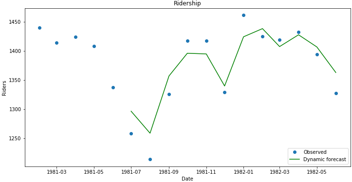
预测值与真实值比较:
| df['forecast']
= results.predict(start = 102, end= 114, dynamic=
True)
df[['riders', 'forecast']].plot(figsize=(12,
6))
plt.savefig('ts_df_predict.png', bbox_inches='tight') |

| npredict
=df['riders']['1982'].shape[0]
fig, ax = plt.subplots(figsize=(12,6))
npre = 12
ax.set(title='Ridership', xlabel='Date', ylabel='Riders')
ax.plot(df.index[-npredict-npre+1:], df.ix[-npredict-npre+1:,
'riders'], 'o', label='Observed')
ax.plot(df.index[-npredict-npre+1:], df.ix[-npredict-npre+1:,
'forecast'], 'g', label='Dynamic forecast')
legend = ax.legend(loc='lower right')
legend.get_frame().set_facecolor('w')
# plt.savefig('ts_predict_compare.png', bbox_inches='tight') |
为了产生针对未来的预测值,我们加入新的时间:
| start
= datetime.datetime.strptime("1982-07-01",
"%Y-%m-%d")
date_list = [start + relativedelta(months=x)
for x in range(0,12)]
future = pd.DataFrame(index=date_list, columns=
df.columns)
df = pd.concat([df, future]) |
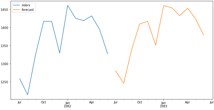
在新加入的时间上来预测未来值:
| df['forecast']
= results.predict(start = 114, end = 125, dynamic=
True)
df[['riders', 'forecast']].ix[-24:].plot(figsize=(12,
8))
#plt.savefig('ts_predict_future.png', bbox_inches='tight') |
|