| БрМЭЦМі: |
ЮФеТНщЩмСЫЩёОЭјТчЕФЛљДЁжЊЪЖЃЌВЂОйР§ЫЕУїСЫШчКЮДюНЈЩёОЭјТчЃЌШчКЮбЕСЗЩёОЭјТчвдМАвЛжжгХЛЏЫуЗЈЫцЛњЬнЖШЯТНЕЃЈSGDЃЉЕШЁЃ
БОЮФРДздгкcsdnЃЌгЩЛ№СњЙћШэМўLucaБрМЁЂЭЦМіЁЃ |
|
ДгСуПЊЪМбЇЯАЩёОЭјТч
ДюНЈЛљБОФЃПщЁЊЩёОдЊ
дкЫЕЩёОЭјТчжЎЧАЃЌЮвУЧЬжТлвЛЯТЩёОдЊЃЈNeuronsЃЉЃЌЫќЪЧЩёОЭјТчЕФЛљБОЕЅдЊЁЃЩёОдЊЯШЛёЕУЪфШыЃЌШЛКѓжДааФГаЉЪ§бЇдЫЫуКѓЃЌдйВњЩњвЛИіЪфГіЁЃБШШчвЛИі2ЪфШыЩёОдЊЕФР§згЃК
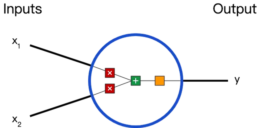
дкетИіЩёОдЊРяЃЌЪфШызмЙВОРњСЫ3ВНЪ§бЇдЫЫуЃЌ
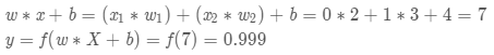
ЯШНЋЪфШыГЫвдШЈжиЃЈweightЃЉЃК
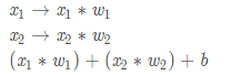
зюКѓОЙ§МЄЛюКЏЪ§ЃЈactivation functionЃЉДІРэЕУЕНЪфГіЃК
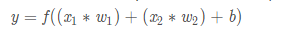
МЄЛюКЏЪ§ЕФзїгУЪЧНЋЮоЯожЦЕФЪфШызЊЛЛЮЊПЩдЄВтаЮЪНЕФЪфГіЁЃвЛжжГЃгУЕФМЄЛюКЏЪ§ЪЧsigmoidКЏЪ§ЃК
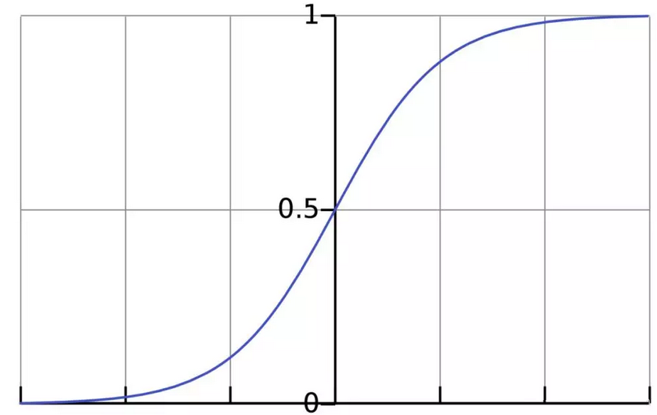
sigmoidКЏЪ§ЕФЪфГіНщгк0КЭ1ЃЌЮвУЧПЩвдРэНтЮЊЫќАб (-Ёо,+Ёо)
ЗЖЮЇФкЕФЪ§бЙЫѕЕН (0, 1)вдФкЁЃе§жЕдНДѓЪфГідННгНќ1ЃЌИКЯђЪ§жЕдНДѓЪфГідННгНќ0ЁЃ
ОйИіР§згЃЌЩЯУцЩёОдЊРяЕФШЈжиКЭЦЋжУШЁШчЯТЪ§жЕЃКw=[0,1];b=4
w=[0,1] ЪЧw1=0,w2=1
ЕФЯђСПаЮЪНаДЗЈЁЃИјЩёОдЊвЛИіЪфШыx=[2,3] ПЩвдгУЯђСПЕуЛ§ЕФаЮЪНАбЩёОдЊЕФЪфГіМЦЫуГіРДЃК
вдЩЯВНжшЕФPythonДњТыЪЧЃК
import numpy
as np
def sigmoid(x):
# our activation function: f(x) = 1 / (1 * e^(-x))
return 1 / (1 + np.exp(-x))
class Neuron():
def __init__(self, weights, bias):
self.weights = weights
self.bias = bias
def feedforward(self, inputs):
# weight inputs, add bias, then use the activation
function
total = np.dot(self.weights, inputs) + self.bias
return sigmoid(total)
weights = np.array([0, 1]) # w1 = 0, w2 = 1
bias = 4
n = Neuron(weights, bias)
# inputs
x = np.array([2, 3]) # x1 = 2, x2 = 3
print(n.feedforward(x)) # 0.9990889488055994 |
ДюНЈЩёОЭјТч
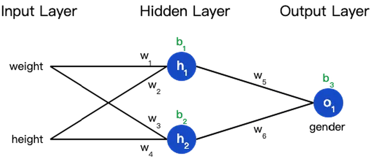
ЩёОЭјТчОЭЪЧАбвЛЖбЩёОдЊСЌНгдквЛЦ№ЃЌЯТУцЪЧвЛИіЩёОЭјТчЕФМђЕЅОйР§ЃК
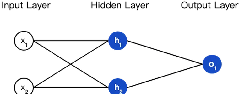
етИіЭјТчга2ИіЪфШыЁЂвЛИіАќКЌ2ИіЩёОдЊЕФвўВиВуЃЈh1КЭh2ЃЉЁЂАќКЌ1ИіЩёОдЊЕФЪфГіВуo1ЁЃ
вўВиВуЪЧМадкЪфШыЪфШыВуКЭЪфГіВужЎМфЕФВПЗжЃЌвЛИіЩёОЭјТчПЩвдгаЖрИівўВиВуЁЃ
АбЩёОдЊЕФЪфШыЯђЧАДЋЕнЛёЕУЪфГіЕФЙ§ГЬГЦЮЊЧАРЁЃЈfeedforwardЃЉЁЃ
ЮвУЧМйЩшЩЯУцЕФЭјТчРяЫљгаЩёОдЊЖМОпгаЯрЭЌЕФШЈжиw=[0,1] КЭЦЋжУb=0
ЃЌМЄЛюКЏЪ§ЖМЪЧsigmoid {sigmoid}sigmoidЃЌФЧУДЮвУЧЛсЕУЕНЪВУДЪфГіФиЃП

вдЯТЪЧЪЕЯжДњТыЃК
class OurNeuralNetworks():
"""
A neural network with:
- 2 inputs
- a hidden layer with 2 neurons (h1, h2)
- an output layer with 1 neuron (o1)
Each neural has the same weights and bias:
- w = [0, 1]
- b = 0
"""
def __init__(self):
weights = np.array([0, 1])
bias = 0
# The Neuron class here is from the previous section
self.h1 = Neuron(weights, bias)
self.h2 = Neuron(weights, bias)
self.o1 = Neuron(weights, bias)
def feedforward(self, x):
out_h1 = self.h1.feedforward(x)
out_h2 = self.h2.feedforward(x)
# The inputs for o1 are the outputs from h1 and
h2
out_o1 = self.o1.feedforward(np.array([out_h1,
out_h2]))
return out_o1
network = OurNeuralNetworks()
x = np.array([2, 3])
print(network.feedforward(x)) # 0.7216325609518421 |
бЕСЗЩёОЭјТч
ЯждкЮвУЧвбОбЇЛсСЫШчКЮДюНЈЩёОЭјТчЃЌЯждкдйРДбЇЯАШчКЮбЕСЗЫќЃЌЦфЪЕетЪЧвЛИігХЛЏЕФЙ§ГЬЁЃ
МйЩшгавЛИіЪ§ОнМЏЃЌАќКЌ4ИіШЫЕФЩэИпЁЂЬхжиКЭадБ№ЃК
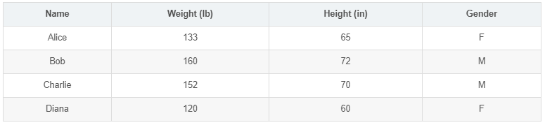
ЯждкЮвУЧЕФФПБъЪЧбЕСЗвЛИіЭјТчЃЌИљОнЬхжиКЭЩэИпРДЭЦВтФГШЫЕФадБ№ЁЃ

ЮЊСЫМђБуЦ№МћЃЌЮвУЧНЋУПИіШЫЕФЩэИпЁЂЬхжиМѕШЅвЛИіЙЬЖЈЪ§жЕЃЌАбадБ№ФаЖЈвхЮЊ1ЁЂадБ№ХЎЖЈвхЮЊ0ЁЃ

дкбЕСЗЩёОЭјТчжЎЧАЃЌЮвУЧашвЊгавЛИіБъзМЖЈвхЫќЕНЕзКУВЛКУЃЌвдБуЮвУЧНјааИФНјЃЌетОЭЪЧЫ№ЪЇЃЈlossЃЉЁЃ
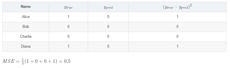
БШШчгУОљЗНЮѓВюЃЈMSEЃЉРДЖЈвхЫ№ЪЇЃК
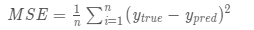
n ЪЧбљБОЕФЪ§СПЃЌдкЩЯУцЕФЪ§ОнМЏжаЪЧ4ЃЛ
y ДњБэШЫЕФадБ№ЃЌФаадЪЧ1ЃЌХЎадЪЧ0ЃЛ
ytrue ЪЧБфСПЕФецЪЕжЕЃЌypredЪЧБфСПЕФдЄВтжЕЁЃ
ЙЫУћЫМвхЃЌОљЗНЮѓВюОЭЪЧЫљгаЪ§ОнЗНВюЕФЦНОљжЕЃЌЮвУЧВЛЗСОЭАбЫќЖЈвхЮЊЫ№ЪЇКЏЪ§ЁЃдЄВтНсЙћдНКУЃЌЫ№ЪЇОЭдНЕЭЃЌбЕСЗЩёОЭјТчОЭЪЧНЋЫ№ЪЇзюаЁЛЏЁЃ
ШчЙћЩЯУцЭјТчЕФЪфГівЛжБЪЧ0ЃЌвВОЭЪЧдЄВтЫљгаШЫЖМЪЧФаадЃЌФЧУДЫ№ЪЇЪЧ
МЦЫуЫ№ЪЇКЏЪ§ЕФДњТыШчЯТЃК
def mse_loss(y_true,
y_pred):
# y_true and y_pred are numpy arrays of the same
length
return ((y_true - y_pred) ** 2).mean()
y_true = np.array([1, 0, 0, 1])
y_pred = np.array([0, 0, 0, 0])
print(mse_loss(y_true, y_pred)) # 0.5 |
МѕЩйЩёОЭјТчЫ№ЪЇ
етИіЩёОЭјТчВЛЙЛКУЃЌЛЙвЊВЛЖЯгХЛЏЃЌОЁСПМѕЩйЫ№ЪЇЁЃЮвУЧжЊЕРЃЌИФБфЭјТчЕФШЈжиКЭЦЋжУПЩвдгАЯьдЄВтжЕЃЌЕЋЮвУЧгІИУдѕУДзіФиЃП
ЮЊСЫМђЕЅЦ№МћЃЌЮвУЧАбЪ§ОнМЏЫѕМѕЕНжЛАќКЌAliceвЛИіШЫЕФЪ§ОнЁЃгкЪЧЫ№ЪЇКЏЪ§ОЭЪЃЯТAliceвЛИіШЫЕФЗНВюЃК

дЄВтжЕЪЧгЩвЛЯЕСаЭјТчШЈжиКЭЦЋжУМЦЫуГіРДЕФЃК
ЫљвдЫ№ЪЇКЏЪ§ЪЕМЪЩЯЪЧАќКЌЖрИіШЈжиЁЂЦЋжУЕФЖрдЊКЏЪ§ЃК
L(w1,w2,w3,w4,w5,w6,b1,b2,b3)
ЃЈзЂвтЃЁЧАЗНИпФмЃЁашвЊФугавЛаЉЛљБОЕФЖрдЊКЏЪ§ЮЂЗжжЊЪЖЃЌБШШчЦЋЕМЪ§ЁЂСДЪНЧѓЕМЗЈдђЁЃЃЉ
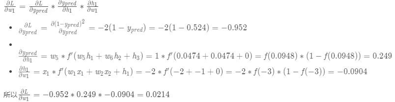
ШчЙћЕїећвЛЯТw1ЃЌЫ№ЪЇКЏЪ§ЪЧЛсБфДѓЛЙЪЧБфаЁЃПЮвУЧашвЊжЊЕРЦЋЕМЪ§ ЪЧе§ЪЧИКВХФмЛиД№етИіЮЪЬтЁЃ ЪЧе§ЪЧИКВХФмЛиД№етИіЮЪЬтЁЃ
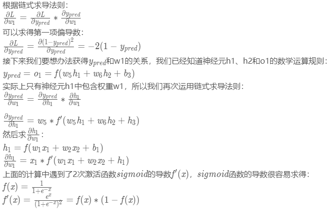
змЕФСДЪНЧѓЕМЙЋЪНЃК
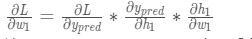
етжжЯђКѓМЦЫуЦЋЕМЪ§ЕФЯЕЭГГЦЮЊЗДЯђДЋВЅЃЈbackpropagationЃЉЁЃ
ЩЯУцЕФЪ§бЇЗћКХЬЋЖрЃЌЯТУцЮвУЧДјШыЪЕМЪЪ§жЕРДМЦЫувЛЯТЁЃh1ЁЂh2КЭo1
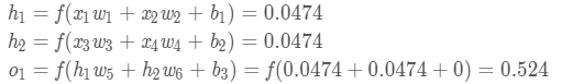
ЩёОЭјТчЕФЪфГіy=0.524ЃЌУЛгаЯдЪОГіЧПСвЕФЪЧФаЃЈ1ЃЉЪЧХЎЃЈ0ЃЉЕФжЄОнЁЃЯждкЕФдЄВтаЇЙћЛЙКмВЛКУЁЃ
етИіНсЙћИцЫпЮвУЧЃКШчЙћдіДѓw1ЃЌЫ№ЪЇКЏЪ§LЛсгавЛИіЗЧГЃаЁЕФдіГЄЁЃ
ЫцЛњЬнЖШЯТНЕ
ЯТУцНЋЪЙгУвЛжжГЦЮЊЫцЛњЬнЖШЯТНЕЃЈSGDЃЉЕФгХЛЏЫуЗЈЃЌРДбЕСЗЭјТчЁЃ
ОЙ§ЧАУцЕФдЫЫуЃЌЮвУЧвбОгаСЫбЕСЗЩёОЭјТчЫљгаЪ§ОнЁЃЕЋЪЧИУШчКЮВйзїЃПSGDЖЈвхСЫИФБфШЈжиКЭЦЋжУЕФЗНЗЈЃК
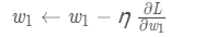
ІЧЪЧвЛИіГЃЪ§ЃЌГЦЮЊбЇЯАТЪЃЈlearning rateЃЉЃЌЫќОіЖЈСЫЮвУЧбЕСЗЭјТчЫйТЪЕФПьТ§ЁЃНЋw1
МѕШЅ ЃЌОЭЕШЕНСЫаТЕФШЈжиw1
ЁЃ ЃЌОЭЕШЕНСЫаТЕФШЈжиw1
ЁЃ
ШчЙћЮвУЧгУетжжЗНЗЈШЅж№ВНИФБфЭјТчЕФШЈжиwКЭЦЋжУbЃЌЫ№ЪЇКЏЪ§ЛсЛКТ§ЕиНЕЕЭЃЌДгЖјИФНјЮвУЧЕФЩёОЭјТчЁЃ
бЕСЗСїГЬШчЯТЃК
ДгЪ§ОнМЏжабЁдёвЛИібљБОЃЛ
МЦЫуЫ№ЪЇКЏЪ§ЖдЫљгаШЈжиКЭЦЋжУЕФЦЋЕМЪ§ЃЛ
ЪЙгУИќаТЙЋЪНИќаТУПИіШЈжиКЭЦЋжУЃЛ
ЛиЕНЕк1ВНЁЃ
PythonДњТыЪЕЯжетИіЙ§ГЬЃК
def sigmoid(x):
# Sigmoid activation function: f(x) = 1 / (1 +
e^(-x))
return 1 / (1 + np.exp(-x))
def deriv_sigmoid(x):
# Derivative of sigmoid: f'(x) = f(x) * (1 - f(x))
fx = sigmoid(x)
return fx * (1 - fx)
def mse_loss(y_true, y_pred):
# y_true and y_pred are numpy arrays of the same
length
return ((y_true - y_pred) ** 2).mean()
class OurNeuralNetwork():
"""
A neural network with:
- 2 inputs
- a hidden layer with 2 neurons (h1, h2)
- an output layer with 1 neuron (o1)
*** DISCLAIMER ***
The code below is intend to be simple and educational,
NOT optimal.
Real neural net code looks nothing like this.
Do NOT use this code.
Instead, read/run it to understand how this specific
network works.
"""
def __init__(self):
# weights
self.w1 = np.random.normal()
self.w2 = np.random.normal()
self.w3 = np.random.normal()
self.w4 = np.random.normal()
self.w5 = np.random.normal()
self.w6 = np.random.normal()
# biases
self.b1 = np.random.normal()
self.b2 = np.random.normal()
self.b3 = np.random.normal()
def feedforward(self, x):
# x is a numpy array with 2 elements, for example
[input1, input2]
h1 = sigmoid(self.w1 * x[0] + self.w2 * x[1] +
self.b1)
h2 = sigmoid(self.w3 * x[0] + self.w4 * x[1] +
self.b2)
o1 = sigmoid(self.w5 * h1 + self.w6 * h2 + self.b3)
return o1
def train(self, data, all_y_trues):
"""
- data is a (n x 2) numpy array, n = # samples
in the dataset.
- all_y_trues is a numpy array with n elements.
Elements in all_y_trues correspond to those in
data.
"""
learn_rate = 0.1
epochs = 1000 # number of times to loop through
the entire dataset
for epoch in range(epochs):
for x, y_true in zip(data, all_y_trues):
# - - - Do a feedforward (we'll need these values
later)
sum_h1 = self.w1 * x[0] + self.w2 * x[1] + self.b1
h1 = sigmoid(sum_h1)
sum_h2 = self.w3 * x[0] + self.w4 * x[1] + self.b2
h2 = sigmoid(sum_h2)
sum_o1 = self.w5 * x[0] + self.w6 * x[1] + self.b3
o1 = sigmoid(sum_o1)
y_pred = o1
# - - - Calculate partial derivatives.
# - - - Naming: d_L_d_w1 represents "partial
L / partial w1"
d_L_d_ypred = -2 * (y_true - y_pred)
# Neuron o1
d_ypred_d_w5 = h1 * deriv_sigmoid(sum_o1)
d_ypred_d_w6 = h2 * deriv_sigmoid(sum_o1)
d_ypred_d_b3 = deriv_sigmoid(sum_o1)
d_ypred_d_h1 = self.w5 * deriv_sigmoid(sum_o1)
d_ypred_d_h2 = self.w6 * deriv_sigmoid(sum_o1)
# Neuron h1
d_h1_d_w1 = x[0] * deriv_sigmoid(sum_h1)
d_h1_d_w2 = x[1] * deriv_sigmoid(sum_h1)
d_h1_d_b1 = deriv_sigmoid(sum_h1)
# Neuron h2
d_h2_d_w3 = x[0] * deriv_sigmoid(sum_h2)
d_h2_d_w4 = x[0] * deriv_sigmoid(sum_h2)
d_h2_d_b2 = deriv_sigmoid(sum_h2)
# - - - update weights and biases
# Neuron o1
self.w5 -= learn_rate * d_L_d_ypred * d_ypred_d_w5
self.w6 -= learn_rate * d_L_d_ypred * d_ypred_d_w6
self.b3 -= learn_rate * d_L_d_ypred * d_ypred_d_b3
# Neuron h1
self.w1 -= learn_rate * d_L_d_ypred * d_ypred_d_h1
* d_h1_d_w1
self.w2 -= learn_rate * d_L_d_ypred * d_ypred_d_h1
* d_h1_d_w2
self.b1 -= learn_rate * d_L_d_ypred * d_ypred_d_h1
* d_h1_d_b1
# Neuron h2
self.w3 -= learn_rate * d_L_d_ypred * d_ypred_d_h2
* d_h2_d_w3
self.w4 -= learn_rate * d_L_d_ypred * d_ypred_d_h2
* d_h2_d_w4
self.b2 -= learn_rate * d_L_d_ypred * d_ypred_d_h2
* d_h2_d_b2
# - - - Calculate total loss at the end of each
epoch
if epoch % 10 == 0:
y_preds = np.apply_along_axis(self.feedforward,
1, data)
loss = mse_loss(all_y_trues, y_preds)
print("Epoch %d loss: %.3f", (epoch,
loss))
# Define dataset
data = np.array([
[-2, -1], # Alice
[25, 6], # Bob
[17, 4], # Charlie
[-15, -6] # diana
])
all_y_trues = np.array([
1, # Alice
0, # Bob
0, # Charlie
1 # diana
])
# Train our neural network!
network = OurNeuralNetwork()
network.train(data, all_y_trues) |
ЫцзХбЇЯАЙ§ГЬЕФНјааЃЌЫ№ЪЇКЏЪ§ж№НЅМѕаЁЁЃ
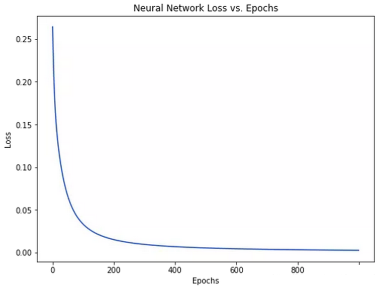
ЯждкЮвУЧПЩвдгУЫќРДЭЦВтГіУПИіШЫЕФадБ№СЫЃК
# Make some predictions
emily = np.array([-7, -3]) # 128 pounds, 63 inches
frank = np.array([20, 2]) # 155 pounds, 68 inches
print("Emily: %.3f" % network.feedforward(emily))
# 0.951 - F
print("Frank: %.3f" % network.feedforward(frank))
# 0.039 - M |
|