| 编辑推荐: |
本文来自于csdn,文章介绍了基本图像处理技术,作者主要使用SciKit-Image
- numpy执行大多数操作。 |
|
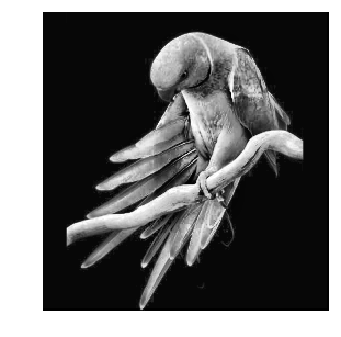
图片亮度转换
让我们先从导入图像开始:
%matplotlib
inline
import imageio
import matplotlib.pyplot as plt
import warnings
import matplotlib.cbook
warnings.filterwarnings("ignore",category
=matplotlib.cbook.mplDeprecation)
pic = imageio.imread('img/parrot.jpg')
plt.figure(figsize = (6,6))
plt.imshow(pic);
plt.axis('off'); |
图片负变换
亮度变换函数在数学上定义为:
其中r是导入图片的像素,s是输出图片的像素。T是一个转换函数,它将r的每个值映射到s的每个值。
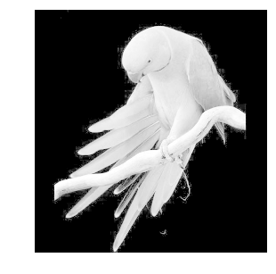
负变换,即变换颠倒。在负变换中,输入图像的每个值从L-1中减去并映射到输出图像上。
在这种情况下,使用以下公式完成转换:
因此每个值减去255,最终效果是,图片原来较亮的部分变暗,较暗的部分变亮,这就产生了负变换。
negative = 255
- pic # neg = (L-1) - img
plt.figure(figsize = (6,6))
plt.imshow(negative);
plt.axis('off'); |
日志转换
日志转换可以由以下公式定义:
其中,s和r是输出和输入图片的像素值,c是常数。值1被添加到输入图片的每个像素值,如果图片中的像素强度为0,则log(0)等于无穷大,添加1的作用是使最小值至少为1。
在对数变换期间,与较高像素值相比,图像中的暗像素被扩展。较高的像素值在日志转换中被压缩,对数变换中的c值可调整增强类型。
%matplotlib
inline
import imageio
import numpy as np
import matplotlib.pyplot as plt
pic = imageio.imread('img/parrot.jpg')
gray = lambda rgb : np.dot(rgb[... , :3] , [0.299
, 0.587, 0.114])
gray = gray(pic)
'''
log transform
-> s = c*log(1+r)
So, we calculate constant c to estimate s
-> c = (L-1)/log(1+|I_max|)
'''
max_ = np.max(gray)
def log_transform():
return (255/np.log(1+max_)) * np.log(1+gray)
plt.figure(figsize = (5,5))
plt.imshow(log_transform(), cmap = plt.get_cmap(name
= 'gray'))
plt.axis('off'); |
Gamma校正
Gamma校正是用于对视频或静止图像系统中的亮度或刺激值进行编码和解码的非线性操作。Gamma校正也称为幂律变换,首先,我们的图片像素强度必须从0,255到0,1.0的范围缩放,通过应用以下等式获得输出的Gamma校正图像:
其中Vi是输入图像,G是gamma值,将输出图像Vo缩放回0-255范围。
gamma值G<1有时被称为编码gamma,并且压缩幂律非线性编码的过程被称为gamma压缩;
Gamma值<1会将图像移向光谱的较暗端。
相反,伽马值G>1被称为解码gamma,并且膨胀幂律非线性应用的过程被称为gamma扩展。Gamma值>1将使图像显得更亮,gamma值G=1对输入图像没有影响:
import imageio
import matplotlib.pyplot as plt
# Gamma encoding
pic = imageio.imread('img/parrot.jpg')
gamma = 2.2 # Gamma < 1 ~ Dark ; Gamma >
1 ~ Bright
gamma_correction = ((pic/255) ** (1/gamma))
plt.figure(figsize = (5,5))
plt.imshow(gamma_correction)
plt.axis('off'); |
Gamma校正的原因
应用Gamma校正的原因是人的眼睛所感知的颜色和亮度与数码相机中的传感器不同。 虽然,数码相机在亮度之间具有线性关系,但人眼是非线性关系。为了解释这种关系,我们应用Gamma校正。
还有一些其他的线性变换函数,比如:
Contrast Stretching
Intensity-Level Slicing
Bit-Plane Slicing
卷积
计算机对图像的处理最终会呈现一个像素值数组。根据图像的分辨率和大小,比如会出现一个32
x 32 x 3的数组,其中3表示RGB值或通道。假设我们有一个PNG格式的彩色图像,它的大小是480
x 480,这代表的数组将是480 * 480 * 3,这些数字中的每一个都在0到255之间,描述了该点的像素强度。
假设我们输入一个32 * 32 * 3的像素值数组,我们该如何理解卷积的概念呢?你可以把它想象为闪烁在图像左上方的手电筒,手电筒照射区域为3
x 3,假设该手电筒滑过输入图像的所有区域。在机器学习中,这个手电筒被称为过滤器或内核,它所照射的区域称为
receptive field 。
现在,此过滤器也是一个数组,其中数字称为权重或参数。需要注意,滤镜的深度必须与输入深度相同,因此滤镜的尺寸为3*3*3。
图像内核或滤镜是一个小矩阵,用于应用可能在Photoshop或Gimp中找到的一些变换,例如模糊、锐化或浮雕等,它们也用于机器学习的功能提取,这是一种用于确定图像重要部分的技术。
现在,让我们将过滤器放在左上角。当滤波器围绕输入图像滑动或卷积时,它将滤波器中的值乘以图像的原始像素值(也称为计算元素乘法)。现在,我们对输入卷上的每个位置重复此过程。下一步是将过滤器向右移动一个步幅,依此类推。输入卷上的每个位置都会生成一个数字。我们也可以选择步幅为2甚至更多,但我们必须保证该数值适合输入图像。
当滤镜滑过所有位置后,我们会发现剩下的是一个30x30x1的数字数组,我们将其称为要素图。我们得到30x30阵列的原因是有300个不同的位置,3x3滤镜可以放在32x32输入图像上。这900个数字映射到30x30阵列。我们可以通过以下方式计算卷积图像:
其中,N和F分别代表输入图像和内核大小,S代表步幅或步长。
假设我们有一个3x3滤波器,在5x5矩阵上进行卷积,根据等式,我们应该得到一个3x3矩阵,技术上称为激活映射或特征映射。
实际上,我们可以使用不止一个过滤器,我们的输出量将是28 * 28 * n(其中n是激活图的数量)。通过使用更多过滤器,我们能够更好保留空间维度。
对于图像矩阵边界上的像素,内核的一些元素可能站在图像矩阵之外,因此不具有来自图像矩阵的任何对应元素。在这种情况下,我们可以消除这些位置的卷积运算,最终出现小于输入的输出矩阵,或者我们可以将填充应用于输入矩阵。
我们可以将自定义统一窗口应用于图像:
%%time
import numpy as np
import imageio
import matplotlib.pyplot as plt
from scipy.signal import convolve2d
def Convolution(image, kernel):
conv_bucket = []
for d in range(image.ndim):
conv_channel = convolve2d(image[:,:,d], kernel,
mode="same", boundary="symm")
conv_bucket.append(conv_channel)
return np.stack(conv_bucket, axis=2).astype("uint8")
kernel_sizes = [9,15,30,60]
fig, axs = plt.subplots(nrows = 1, ncols = len(kernel_sizes),
figsize=(15,15));
pic = imageio.imread('img:/parrot.jpg')
for k, ax in zip(kernel_sizes, axs):
kernel = np.ones((k,k))
kernel /= np.sum(kernel)
ax.imshow(Convolution(pic, kernel));
ax.set_title("Convolved By Kernel: {}".format(k));
ax.set_axis_off();
Wall time: 43.5 s |
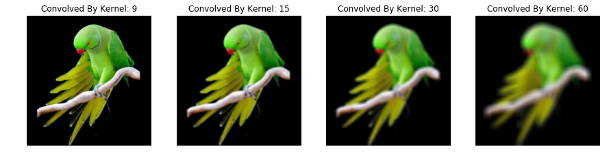
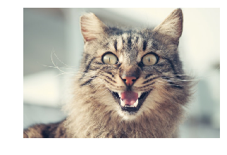
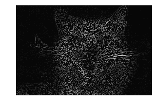
轮廓内核(又名“边缘”内核)用于突出显示像素值之间的差异,亮度接近的相邻像素旁边的像素在新图像中将显示为黑色,而差异性较大的相邻像素的旁边像素将显示为白色。
%%time
from skimage import color
from skimage import exposure
import numpy as np
import imageio
import matplotlib.pyplot as plt
# import image
pic = imageio.imread('img/crazycat.jpeg')
plt.figure(figsize = (5,5))
plt.imshow(pic)
plt.axis('off');
Wall time: 34.9 ms |
# Convert the
image to grayscale
img = color.rgb2gray(pic)
# outline kernel - used for edge detection
kernel = np.array([[-1,-1,-1],
[-1,8,-1],
[-1,-1,-1]])
# we use 'valid' which means we do not add zero
padding to our image
edges = convolve2d(img, kernel, mode = 'valid')
# Adjust the contrast of the filtered image by
applying Histogram Equalization
edges_equalized = exposure.equalize_adapthist
(edges/np.max(np.abs(edges)),
clip_limit = 0.03)
# plot the edges_clipped
plt.figure(figsize = (5,5))
plt.imshow(edges_equalized, cmap='gray')
plt.axis('off'); |
让我们用不同类型的过滤器试一下,比如Sharpen Kernel。锐化内核强调相邻像素值的之间差异,这会让图像看起来更生动。让我们将边缘检测内核应用于锐化内核的输出,并使用
box blur filter进一步标准化。
%%time
from skimage import color
from skimage import exposure
from scipy.signal import convolve2d
import numpy as np
import imageio
import matplotlib.pyplot as plt
# Convert the image to grayscale
img = color.rgb2gray(pic)
# apply sharpen filter to the original image
sharpen_kernel = np.array([[0,-1,0],
[-1,5,-1],
[0,-1,0]])
image_sharpen = convolve2d(img, sharpen_kernel,
mode = 'valid')
# apply edge kernel to the output of the sharpen
kernel
edge_kernel = np.array([[-1,-1,-1],
[-1,8,-1],
[-1,-1,-1]])
edges = convolve2d(image_sharpen, edge_kernel,
mode = 'valid')
# apply normalize box blur filter to the edge
detection filtered image
blur_kernel = np.array([[1,1,1],
[1,1,1],
[1,1,1]])/9.0;
denoised = convolve2d(edges, blur_kernel, mode
= 'valid')
# Adjust the contrast of the filtered image by
applying Histogram Equalization
denoised_equalized = exposure.equalize_adapthist
(denoised/np.max(np.abs(denoised)),
clip_limit=0.03)
plt.figure(figsize = (5,5))
plt.imshow(denoised_equalized, cmap='gray')
plt.axis('off')
plt.show() |

为了模糊图像,可以使用大量不同的窗口和功能。 其中最常见的是Gaussian
window。为了解它对图像的作用,让我们将此过滤器应用于图像。
%%time
from skimage import color
from skimage import exposure
from scipy.signal import convolve2d
import numpy as np
import imageio
import matplotlib.pyplot as plt
# import image
pic = imageio.imread('img/parrot.jpg')
# Convert the image to grayscale
img = color.rgb2gray(pic)
# gaussian kernel - used for blurring
kernel = np.array([[1,2,1],
[2,4,2],
[1,2,1]])
kernel = kernel / np.sum(kernel)
# we use 'valid' which means we do not add zero
padding to our image
edges = convolve2d(img, kernel, mode = 'valid')
# Adjust the contrast of the filtered image by
applying Histogram Equalization
edges_equalized = exposure.equalize_adapthist
(edges/np.max(np.abs(edges)),
clip_limit = 0.03)
# plot the edges_clipped
plt.figure(figsize = (5,5))
plt.imshow(edges_equalized, cmap='gray')
plt.axis('off')
plt.show() |
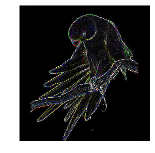
通过使用更多窗户,可以提取不同种类的信息。 Sobel kernels 仅用于显示特定方向上相邻像素值的差异,尝试使用内核函数沿一个方向近似图像的梯度。
通过在X和Y方向移动,我们可以得到图像中每个颜色的梯度图。
%%time
from skimage import color
from skimage import exposure
from scipy.signal import convolve2d
import numpy as np
import imageio
import matplotlib.pyplot as plt
# import image
pic = imageio.imread('img/parrot.jpg')
# right sobel
sobel_x = np.c_[
[-1,0,1],
[-2,0,2],
[-1,0,1]
]
# top sobel
sobel_y = np.c_[
[1,2,1],
[0,0,0],
[-1,-2,-1]
]
ims = []
for i in range(3):
sx = convolve2d(pic[:,:,i], sobel_x, mode="same",
boundary="symm")
sy = convolve2d(pic[:,:,i], sobel_y, mode="same",
boundary="symm")
ims.append(np.sqrt(sx*sx + sy*sy))
img_conv = np.stack(ims, axis=2).astype("uint8")
plt.figure(figsize = (6,5))
plt.axis('off')
plt.imshow(img_conv); |
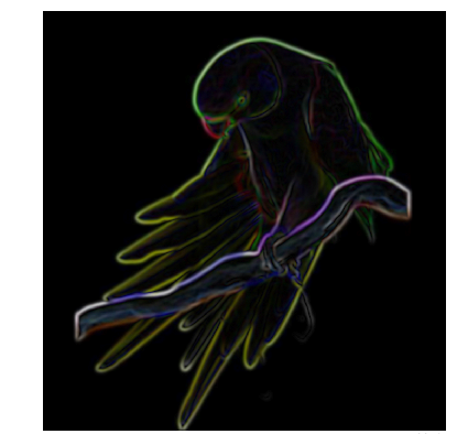
至于降噪,我们通常使用类似Gaussian Filter的滤波器,这是一种数字滤波技术,通常用于图片降噪。通过将Gaussian
Filter和gradient finding操作结合在一起,我们可以生成一些类似于原始图像并以有趣方式扭曲的奇怪图案。
%%time
from scipy.signal import convolve2d
from scipy.ndimage import (median_filter, gaussian_filter)
import numpy as np
import imageio
import matplotlib.pyplot as plt
def gaussain_filter_(img):
"""
Applies a median filer to all channels
"""
ims = []
for d in range(3):
img_conv_d = gaussian_filter(img[:,:,d], sigma
= 4)
ims.append(img_conv_d)
return np.stack(ims, axis=2).astype("uint8")
filtered_img = gaussain_filter_(pic)
# right sobel
sobel_x = np.c_[
[-1,0,1],
[-2,0,2],
[-1,0,1]
]
# top sobel
sobel_y = np.c_[
[1,2,1],
[0,0,0],
[-1,-2,-1]
]
ims = []
for d in range(3):
sx = convolve2d(filtered_img[:,:,d], sobel_x,
mode="same", boundary="symm")
sy = convolve2d(filtered_img[:,:,d], sobel_y,
mode="same", boundary="symm")
ims.append(np.sqrt(sx*sx + sy*sy))
img_conv = np.stack(ims, axis=2).astype("uint8")
plt.figure(figsize=(7,7))
plt.axis('off')
plt.imshow(img_conv); |
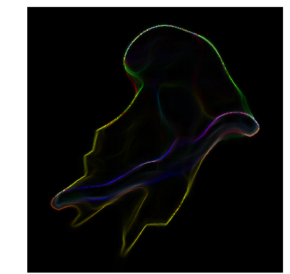
现在,让我们来看看使用Median filter 可以对图像产生什么效果。
%%time
from scipy.signal import convolve2d
from scipy.ndimage import (median_filter, gaussian_filter)
import numpy as np
import imageio
import matplotlib.pyplot as plt
def median_filter_(img, mask):
"""
Applies a median filer to all channels
"""
ims = []
for d in range(3):
img_conv_d = median_filter(img[:,:,d], size=(mask,mask))
ims.append(img_conv_d)
return np.stack(ims, axis=2).astype("uint8")
filtered_img = median_filter_(pic, 80)
# right sobel
sobel_x = np.c_[
[-1,0,1],
[-2,0,2],
[-1,0,1]
]
# top sobel
sobel_y = np.c_[
[1,2,1],
[0,0,0],
[-1,-2,-1]
]
ims = []
for d in range(3):
sx = convolve2d(filtered_img[:,:,d], sobel_x,
mode="same", boundary="symm")
sy = convolve2d(filtered_img[:,:,d], sobel_y,
mode="same", boundary="symm")
ims.append(np.sqrt(sx*sx + sy*sy))
img_conv = np.stack(ims, axis=2).astype("uint8")
plt.figure(figsize=(7,7))
plt.axis('off')
plt.imshow(img_conv);
|
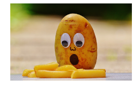
阈值之 Ostu方法
阈值处理是图像处理中非常基本的操作,将灰度图像转换为单色是常见的图像处理任务。而且,一个好的算法总是以良好的基础开始!
Otsu阈值处理是一种简单而有效的全局自动阈值处理方法,用于二值化灰度图像,如前景和背景。在图像处理中,Otsu的阈值处理方法(1979)基于直方图的形状自动二值化水平决定,完全基于对图像直方图执行的计算。
该算法假设图像由两个基本类组成:前景和背景,计算最小阈值并最小化两类的类方差加权。
算法
如果我们在这个简单的逐步算法中加入一点数学,那么这种解释就会发生变化:
计算每个强度级别的直方图和概率。
设置初始wi和μi。
从阈值t = 0到t = L-1:
oupdate:wi和μi
ocompute:σ_b** 2(t)
所需阈值对应于σ_b** 2(t)的最大值。
import numpy
as np
import imageio
import matplotlib.pyplot as plt
pic = imageio.imread('img/potato.jpeg')
plt.figure(figsize=(7,7))
plt.axis('off')
plt.imshow(pic); |
def otsu_threshold(im):
# Compute histogram and probabilities of each
intensity level
pixel_counts = [np.sum(im == i) for i in range(256)]
# Initialization
s_max = (0,0)
for threshold in range(256):
# update
w_0 = sum(pixel_counts[:threshold])
w_1 = sum(pixel_counts[threshold:])
mu_0 = sum([i * pixel_counts[i] for i in range(0,threshold)])
/ w_0 if w_0 > 0 else 0
mu_1 = sum([i * pixel_counts[i] for i in range(threshold,
256)]) / w_1 if w_1 > 0 else 0
# calculate - inter class variance
s = w_0 * w_1 * (mu_0 - mu_1) ** 2
if s > s_max[1]:
s_max = (threshold, s)
return s_max[0] |
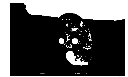
如果可以假设直方图具有双峰分布并且两峰之间具有深且尖锐的谷,则Otsu的方法会表现更优。如果前景与背景差异较小,则直方图不会呈现双峰性。
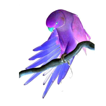
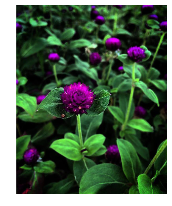
K-Means聚类
K-Means聚类是一种矢量量化方法,最初来自信号处理,是数据挖掘中聚类分析的常用方法。
在Otsu阈值处理中,我们找到了最小化段内像素方差的阈值。 因此,我们不是从灰度图像中寻找阈值,而是在颜色空间中寻找聚类,通过这样做,我们最终得到了K-means聚类。
from sklearn
import cluster
import matplotlib.pyplot as plt
# load image
pic = imageio.imread('img/purple.jpg')
plt.figure(figsize=(7,7))
plt.imshow(pic)
plt.axis('off');
|
为了聚类图像,我们需要将其转换为二维数组。
接下来,我们使用scikit-learn方法创建集群,传递n_clusters
5以形成五个集群。聚类出现在生成图像中,将其分为五个部分,每部分的颜色不同。
%%time
# fit on the image with cluster five
kmeans_cluster = cluster.KMeans(n_clusters=5)
kmeans_cluster.fit(pic_2d)
cluster_centers = kmeans_cluster.cluster_centers_
cluster_labels = kmeans_cluster.labels_
|
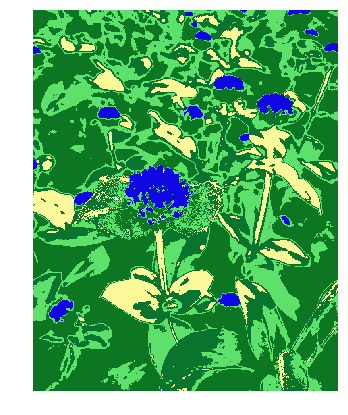
一旦形成了簇,我们就可以使用簇中心和标签重新创建图像,以显示具有分组模式的图像。
直线检测之霍夫变换
如果我们能够以数学形式表示该形状,则霍夫变换是一种用于检测任何形状的流行技术。它可以检测形状,即使它被破坏或扭曲一点点。
我们不会过于深入分析霍夫变换的机制。
算法
Corner或边缘检测
ρ范围和θ范围创建
ρ:Dmax至Dmax
θ:90到90
霍夫变换
2D数组的行数等于ρ值的数量,列数等于θ值的数量。
在累加器中投票
对于每个边缘点和θ值,找到最接近的ρ值并在累加器中递增该索引。
累加器中的局部最大值指示输入图像中最突出的线的参数。
def hough_line(img):
# Rho and Theta ranges
thetas = np.deg2rad(np.arange(-90.0, 90.0))
width, height = img.shape
diag_len = int(np.ceil(np.sqrt(width * width +
height * height))) # Dmax
rhos = np.linspace(-diag_len, diag_len, diag_len
* 2.0)
# Cache some resuable values
cos_t = np.cos(thetas)
sin_t = np.sin(thetas)
num_thetas = len(thetas)
# Hough accumulator array of theta vs rho
accumulator = np.zeros((2 * diag_len, num_thetas),
dtype=np.uint64)
y_idxs, x_idxs = np.nonzero(img) # (row, col)
indexes to edges
# Vote in the hough accumulator
for i in range(len(x_idxs)):
x = x_idxs[i]
y = y_idxs[i]
for t_idx in range(num_thetas):
# Calculate rho. diag_len is added for a positive
index
rho = round(x * cos_t[t_idx] + y * sin_t[t_idx])
+ diag_len
accumulator[rho, t_idx] += 1
return accumulator, thetas, rhos |
边缘检测
边缘检测是一种用于查找图像内对象边界的图像处理技术。它的工作原理是检测亮度的不连续性。
常见的边缘检测算法包括
Sobel
Canny
Prewitt
Roberts
fuzzy logic methods
在这里,我们将介绍一种最流行的方法,即Canny Edge Detection(Canny边缘检测)。
Canny边缘检测
一种能够检测图像中较宽范围边缘的多级边缘检测操作,Canny边缘检测算法可以分解为5步:
应用高斯滤波器
找出强度梯度
应用非极大值抑制
应用双阈值
通过滞后性门限跟踪边缘线
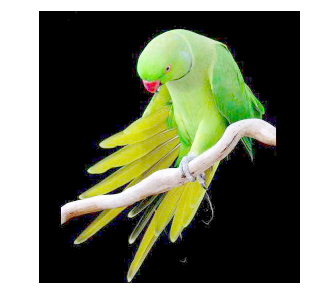
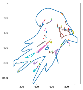
图片矢量之轮廓跟踪
使用Scikit-Image,我们可以使用轮廓跟踪算法提取图片边缘路径(勾勒图片轮廓),这可以控制最终路径遵循原始位图的形状。
from sklearn.cluster
import KMeans
import matplotlib.pyplot as plt
from skimage import measure
import numpy as np
import imageio
pic = imageio.imread('img/parrot.jpg')
h,w = pic.shape[:2]
im_small_long = pic.reshape((h * w, 3))
im_small_wide = im_small_long.reshape((h,w,3))
km = KMeans(n_clusters=2)
km.fit(im_small_long)
seg = np.asarray([(1 if i == 1 else 0)
for i in km.labels_]).reshape((h,w))
contours = measure.find_contours(seg, 0.5, fully_connected="high")
simplified_contours = [measure.approximate_polygon(c,
tolerance=5)
for c in contours]
plt.figure(figsize=(5,10))
for n, contour in enumerate(simplified_contours):
plt.plot(contour[:, 1], contour[:, 0], linewidth=2)
plt.ylim(h,0)
plt.axes().set_aspect('equal') |
图像压缩之堆叠自编码器
Autoencoder是一种数据压缩算法,其中压缩和解压缩功能是:
Data-specific
Lossy
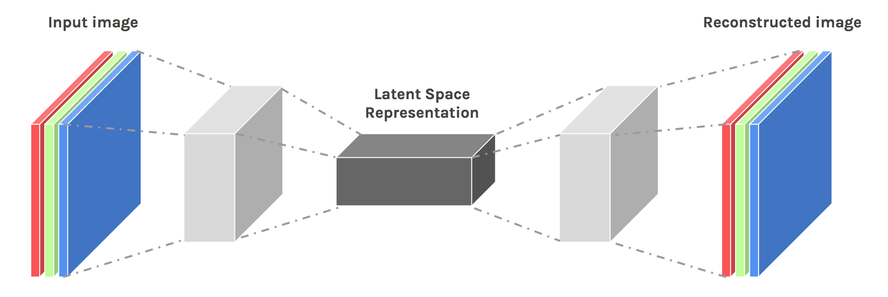
以下为具体实现代码:
import numpy
as np
import matplotlib.pyplot as plt
import tensorflow as tf
from tensorflow.examples.tutorials.mnist import
input_data
mnist = input_data.read_data_sets("MNIST_data",one_hot=True)
# Parameter
num_inputs = 784 # 28*28
neurons_hid1 = 392
neurons_hid2 = 196
neurons_hid3 = neurons_hid1 # Decoder Begins
num_outputs = num_inputs
learning_rate = 0.01
# activation function
actf = tf.nn.relu
# place holder
X = tf.placeholder(tf.float32, shape=[None, num_inputs])
# Weights
initializer = tf.variance_scaling_initializer()
w1 = tf.Variable(initializer([num_inputs, neurons_hid1]),
dtype=tf.float32)
w2 = tf.Variable(initializer([neurons_hid1, neurons_hid2]),
dtype=tf.float32)
w3 = tf.Variable(initializer([neurons_hid2, neurons_hid3]),
dtype=tf.float32)
w4 = tf.Variable(initializer([neurons_hid3, num_outputs]),
dtype=tf.float32)
# Biases
b1 = tf.Variable(tf.zeros(neurons_hid1))
b2 = tf.Variable(tf.zeros(neurons_hid2))
b3 = tf.Variable(tf.zeros(neurons_hid3))
b4 = tf.Variable(tf.zeros(num_outputs))
# Activation Function and Layers
act_func = tf.nn.relu
hid_layer1 = act_func(tf.matmul(X, w1) + b1)
hid_layer2 = act_func(tf.matmul(hid_layer1, w2)
+ b2)
hid_layer3 = act_func(tf.matmul(hid_layer2, w3)
+ b3)
output_layer = tf.matmul(hid_layer3, w4) + b4
# Loss Function
loss = tf.reduce_mean(tf.square(output_layer -
X))
# Optimizer
optimizer = tf.train.AdamOptimizer(learning_rate)
train = optimizer.minimize(loss)
# Intialize Variables
init = tf.global_variables_initializer()
saver = tf.train.Saver()
num_epochs = 5
batch_size = 150
with tf.Session() as sess:
sess.run(init)
# Epoch == Entire Training Set
for epoch in range(num_epochs):
num_batches = mnist.train.num_examples // batch_size
# 150 batch size
for iteration in range(num_batches):
X_batch, y_batch = mnist.train.next_batch(batch_size)
sess.run(train, feed_dict={X: X_batch})
training_loss = loss.eval(feed_dict={X: X_batch})
print("Epoch {} Complete. Training Loss:
{}".format(epoch,training_loss))
saver.save(sess, "./stacked_autoencoder.ckpt")
# Test Autoencoder output on Test Data
num_test_images = 10
with tf.Session() as sess:
saver.restore(sess,"./stacked_autoencoder.ckpt")
results = output_layer.eval(feed_dict={X:mnist.test.images[:num_test_images]})
Extracting MNIST_data\train-images-idx3-ubyte.gz
Extracting MNIST_data\train-labels-idx1-ubyte.gz
Extracting MNIST_data\t10k-images-idx3-ubyte.gz
Extracting MNIST_data\t10k-labels-idx1-ubyte.gz
Epoch 0 Complete. Training Loss: 0.023349963128566742
Epoch 1 Complete. Training Loss: 0.022537199780344963
Epoch 2 Complete. Training Loss: 0.0200303066521883
Epoch 3 Complete. Training Loss: 0.021327141672372818
Epoch 4 Complete. Training Loss: 0.019387174397706985
INFO:tensorflow:Restoring parameters from ./stacked_autoencoder.ckpt |
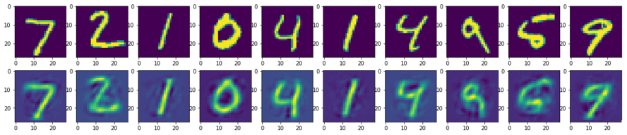
第一行加载MNIST训练集,第二行使用自编码器进行编码和解码,之后重构训练集。但是,重建图像中缺少大量信息。因此,自编码器不如其他压缩技术好,但作为一门正在快速增长中的技术,其未来还会出现很多进步。
(代码下载可访问Github地址:https://github.com/iphton/Image-Processing-in-Python) |