| 编辑推荐: |
本文来自于网络,文章详细介绍了使用Python实现机器学习算法的损失函数、反向传播过程等相关知识。
|
|
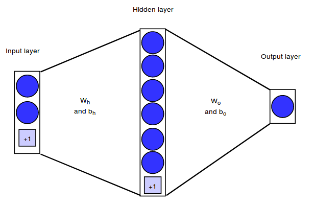
在这一章节里,我们将实现一个简单的神经网络架构,将 2 维的输入向量映射成二进制输出值。我们的神经网络有
2 个输入神经元,含 6 个隐藏神经元隐藏层及 1 个输出神经元。
我们将通过层之间的权重矩阵来表示神经网络结构。在下面的例子中,输入层和隐藏层之间的权重矩阵将被表示为Wh,隐藏层和输出层之间的权重矩阵为Wo。除了连接神经元的权重向量外,每个隐藏和输出的神经元都会有一个大小为
1 的偏置量。
我们的训练集由 m = 750 个样本组成。因此,我们的矩阵维度如下:
训练集维度: X = (750,2)
目标维度: Y = (750,1)
Wh维度:(m,nhidden) = (2,6)
bh维度:(bias
vector):(1,nhidden) = (1,6)
Wo维度: (nhidden,noutput)=
(6,1)
bo维度:(bias
vector):(1,noutput) = (1,1)
损失函数
我们使用与 Logistic 回归算法相同的损失函数:
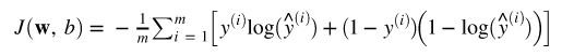
对于多类别的分类任务,我们将使用这个函数的通用形式作为损失函数,称之为分类交叉熵函数。
训练
我们将用梯度下降法来训练我们的神经网络,并通过反向传播法来计算所需的偏导数。训练过程主要有以下几个步骤:
1. 初始化参数(即权重量和偏差量)
2. 重复以下过程,直到收敛:
通过网络传播当前输入的批次大小,并计算所有隐藏和输出单元的激活值和输出值。
针对每个参数计算其对损失函数的偏导数
更新参数
前向传播过程
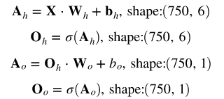
首先,我们计算网络中每个单元的激活值和输出值。为了加速这个过程的实现,我们不会单独为每个输入样本执行此操作,而是通过矢量化对所有样本一次性进行处理。其中:
Ah表示对所有训练样本激活隐层单元的矩阵
Oh表示对所有训练样本输出隐层单位的矩阵
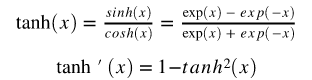
隐层神经元将使用 tanh 函数作为其激活函数:
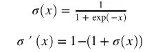
输出层神经元将使用 sigmoid 函数作为激活函数:
激活值和输出值计算如下(·表示点乘):
反向传播过程
为了计算权重向量的更新值,我们需要计算每个神经元对损失函数的偏导数。这里不会给出这些公式的推导,你会在其他网站上找到很多更好的解释。
对于输出神经元,梯度计算如下(矩阵符号):
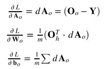
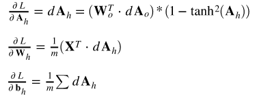
对于输入和隐层的权重矩阵,梯度计算如下:
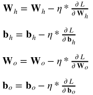
权重更新
In [3]:
import numpy
as np
import pandas as pd
import matplotlib.pyplot as plt
from sklearn.datasets import make_circles
from sklearn.model_selection import train_test_split
np.random.seed(123)
% matplotlib inline |
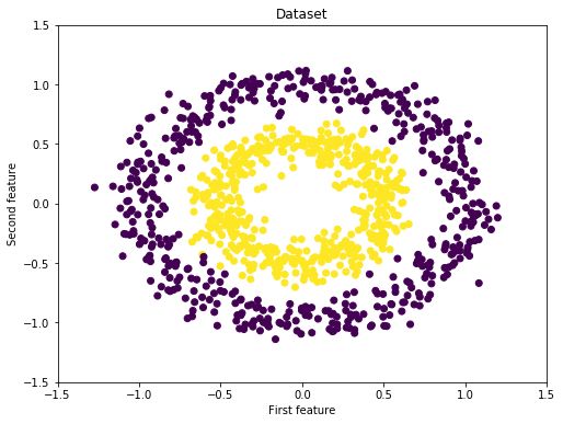
数据集
In [4]:
X, y = make_circles(n_samples=1000,
factor=0.5, noise=.1)
fig = plt.figure(figsize=(8,6))
plt.scatter(X[:,0], X[:,1], c=y)
plt.xlim([-1.5, 1.5])
plt.ylim([-1.5, 1.5])
plt.title("Dataset")
plt.xlabel("First feature")
plt.ylabel("Second feature")
plt.show() |
In [5]:
# reshape targets
to get column vector with shape (n_samples, 1)
y_true = y[:, np.newaxis]
# Split the data into a training and test set
X_train, X_test, y_train, y_test = train_test_split(X,
y_true)
print(f'Shape X_train: {X_train.shape}')
print(f'Shape y_train: {y_train.shape}')
print(f'Shape X_test: {X_test.shape}')
print(f'Shape y_test: {y_test.shape}') |
Shape X_train: (750, 2)
Shape y_train: (750, 1)
Shape X_test: (250, 2)
Shape y_test: (250, 1)
Neural Network Class
class NeuralNet():
def __init__(self, n_inputs, n_outputs, n_hidden):
self.n_inputs = n_inputs
self.n_outputs = n_outputs
self.hidden = n_hidden
# Initialize weight matrices and bias vectors
self.W_h = np.random.randn(self.n_inputs, self.hidden)
self.b_h = np.zeros((1, self.hidden))
self.W_o = np.random.randn(self.hidden, self.n_outputs)
self.b_o = np.zeros((1, self.n_outputs))
def sigmoid(self, a):
return 1 / (1 + np.exp(-a))
def forward_pass(self, X):
"""
Propagates the given input X forward through the
net.
Returns:
A_h: matrix with activations of all hidden neurons
for all input examples
O_h: matrix with outputs of all hidden neurons
for all input examples
A_o: matrix with activations of all output neurons
for all input examples
O_o: matrix with outputs of all output neurons
for all input examples
"""
# Compute activations and outputs of hidden units
A_h = np.dot(X, self.W_h) + self.b_h
O_h = np.tanh(A_h)
# Compute activations and outputs of output units
A_o = np.dot(O_h, self.W_o) + self.b_o
O_o = self.sigmoid(A_o)
outputs = {
"A_h": A_h,
"A_o":
A_o,
"O_h": O_h,
"O_o":
O_o,
}
return outputs
def cost(self, y_true, y_predict, n_samples):
"""
Computes and returns the cost over all examples
"""
# same cost function as in logistic regression
cost = (- 1 / n_samples) * np.sum(y_true * np.log(y_predict)
+ (1 - y_true) * (np.log(1 - y_predict)))
cost = np.squeeze(cost)
assert isinstance(cost, float)
return cost
def backward_pass(self, X, Y, n_samples, outputs):
"""
Propagates the errors backward through the net.
Returns:
dW_h: partial derivatives of loss function w.r.t
hidden weights
db_h: partial derivatives of loss function w.r.t
hidden bias
dW_o: partial derivatives of loss function w.r.t
output weights
db_o: partial derivatives of loss function w.r.t
output bias
"""
dA_o = (outputs["O_o"] - Y)
dW_o = (1 / n_samples) * np.dot(outputs["O_h"].T,
dA_o)
db_o = (1 / n_samples) * np.sum(dA_o)
dA_h = (np.dot(dA_o, self.W_o.T)) * (1 - np.power(outputs["O_h"],
2))
dW_h = (1 / n_samples) * np.dot(X.T, dA_h)
db_h = (1 / n_samples) * np.sum(dA_h)
gradients = {
"dW_o": dW_o,
"db_o": db_o,
"dW_h":
dW_h,
"db_h": db_h,
}
return gradients
def update_weights(self, gradients, eta):
"""
Updates the model parameters using a fixed learning
rate
"""
self.W_o = self.W_o - eta * gradients["dW_o"]
self.W_h = self.W_h - eta * gradients["dW_h"]
self.b_o = self.b_o - eta * gradients["db_o"]
self.b_h = self.b_h - eta * gradients["db_h"]
def train(self, X, y, n_iters=500, eta=0.3):
"""
Trains the neural net on the given input data
"""
n_samples, _ = X.shape
for i in range(n_iters):
outputs = self.forward_pass(X)
cost = self.cost(y, outputs["O_o"],
n_samples=n_samples)
gradients = self.backward_pass(X, y, n_samples,
outputs)
if i % 100 == 0:
print(f'Cost at iteration {i}: {np.round(cost,
4)}')
self.update_weights(gradients, eta)
def predict(self, X):
"""
Computes and returns network predictions for given
dataset
"""
outputs = self.forward_pass(X)
y_pred = [1 if elem >= 0.5 else 0 for elem
in outputs["O_o"]]
return np.array(y_pred)[:, np.newaxis] |
初始化并训练神经网络
nn = NeuralNet(n_inputs=2,
n_hidden=6, n_outputs=1)
print("Shape of weight matrices and bias
vectors:")
print(f'W_h shape: {nn.W_h.shape}')
print(f'b_h shape: {nn.b_h.shape}')
print(f'W_o shape: {nn.W_o.shape}')
print(f'b_o shape: {nn.b_o.shape}')
print()
print("Training:")
nn.train(X_train, y_train, n_iters=2000, eta=0.7) |
Shape of weight matrices and bias vectors:
W_h shape: (2, 6)
b_h shape: (1, 6)
W_o shape: (6, 1)
b_o shape: (1, 1)
Training:
Cost at iteration 0: 1.0872
Cost at iteration 100: 0.2723
Cost at iteration 200: 0.1712
Cost at iteration 300: 0.1386
Cost at iteration 400: 0.1208
Cost at iteration 500: 0.1084
Cost at iteration 600: 0.0986
Cost at iteration 700: 0.0907
Cost at iteration 800: 0.0841
Cost at iteration 900: 0.0785
Cost at iteration 1000: 0.0739
Cost at iteration 1100: 0.0699
Cost at iteration 1200: 0.0665
Cost at iteration 1300: 0.0635
Cost at iteration 1400: 0.061
Cost at iteration 1500: 0.0587
Cost at iteration 1600: 0.0566
Cost at iteration 1700: 0.0547
Cost at iteration 1800: 0.0531
Cost at iteration 1900: 0.0515
测试神经网络
n_test_samples,
_ = X_test.shape
y_predict = nn.predict(X_test)
print(f"Classification accuracy on test set:
{(np.sum(y_predict == y_test)/n_test_samples)*100}
%") |
Classification accuracy on test set: 98.4 %
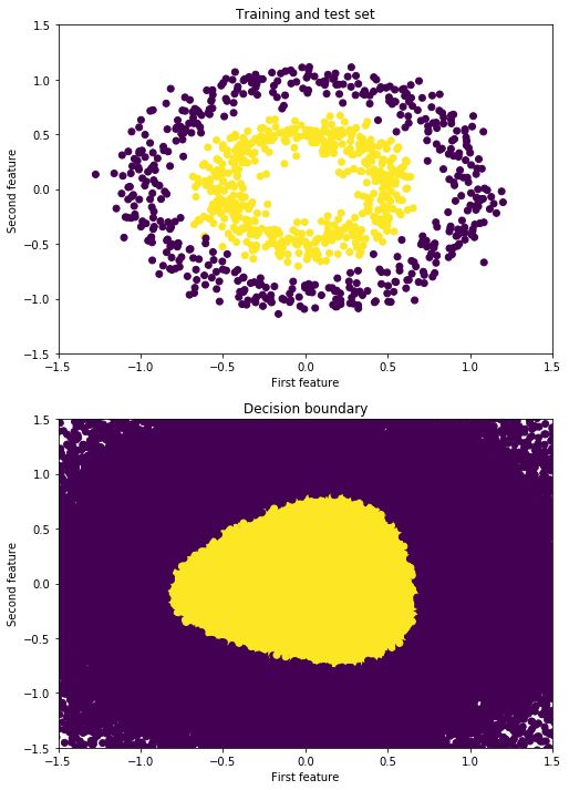
可视化决策边界
X_temp, y_temp
= make_circles(n_samples=60000, noise=.5)
y_predict_temp = nn.predict(X_temp)
y_predict_temp = np.ravel(y_predict_temp) |
fig = plt.figure(figsize=(8,12))
ax = fig.add_subplot(2,1,1)
plt.scatter(X[:,0], X[:,1], c=y)
plt.xlim([-1.5, 1.5])
plt.ylim([-1.5, 1.5])
plt.xlabel("First feature")
plt.ylabel("Second feature")
plt.title("Training and test set")
ax = fig.add_subplot(2,1,2)
plt.scatter(X_temp[:,0], X_temp[:,1], c=y_predict_temp)
plt.xlim([-1.5, 1.5])
plt.ylim([-1.5, 1.5])
plt.xlabel("First feature")
plt.ylabel("Second feature")
plt.title("Decision boundary") |
Out[11]:Text(0.5,1,'Decision boundary')
|