| 编辑推荐: |
篇博文主要介绍逻辑回归(logistic regression),首先介绍相关的基础概念和原理,然后通过Python代码实现逻辑回归的二分类问题。特别强调,其中大多理论知识来源于《统计学习方法_李航》和斯坦福课程翻译笔记以及Coursera机器学习课程。
本文来自于csdn,由火龙果软件Anna编辑、推荐。 |
|
本篇博文的理论知识都来自于吴大大的Coursera机器学习课程,人家讲的深入浅出,我就不一一赘述,只是简单概括一下以及记一下自己的见解。
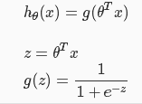
1.逻辑回归假设函数
逻辑回归一般用于分类问题较多,但是叫做“regression”,而线性回归一般不建议用于分类,因为输出的y的值可能超出0/1范围。这也就是为什么逻辑回归假设函数里面有sigmoid函数的原因了。
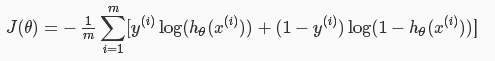
2.成本函数
逻辑回归问题不在采用“最小均方”误差,因为里面含有非线性的sigmiod函数,使得成本函数J不再是一个平滑的“碗”,容易导致“局部最优”,所以采用如下cost
function:
3.参数学习(梯度下降)
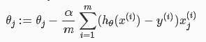
你会发现,这个跟线性回归模型的梯度下降表达上一模一样,但是,你要知道,其中的h(x)是不一样的!
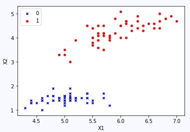
4.Python代码实现
先看一下数据集,这是一种花的数据集,只取X中的两个特征(x1,x2),对于y中的两个类别(0,1)
from sklearn.datasets
import load_iris
import matplotlib.pyplot as plt
import numpy as np
iris = load_iris()
data = iris.data
target = iris.target
#print data[:10]
#print target[10:]
X = data[0:100,[0,2]]
y = target[0:100]
print X[:5]
print y[-5:]
label = np.array(y)
index_0 = np.where(label==0)
plt.scatter(X[index_0,0],X[index_0,1], marker='x',color
= 'b',label = '0',s = 15)
index_1 =np.where(label==1)
plt.scatter(X[index_1,0],X[index_1,1], marker='o',color
= 'r',label = '1',s = 15)
plt.xlabel('X1')
plt.ylabel('X2')
plt.legend(loc = 'upper left')
plt.show() |
编写逻辑回归模型的类
import numpy
as np
class logistic(object):
def __init__(self):
self.W = None
def train(self,X,y,learn_rate = 0.01,num_iters
= 5000):
num_train,num_feature = X.shape
#init the weight
self.W = 0.001*np.random.randn(num_feature,1).reshape((-1,1))
loss = []
for i in range(num_iters):
error,dW = self.compute_loss(X,y)
self.W += -learn_rate*dW
loss.append(error)
if i%200==0:
print 'i=%d,error=%f' %(i,error)
return loss
def compute_loss(self,X,y):
num_train = X.shape[0]
h = self.output(X)
loss = -np.sum((y*np.log(h) + (1-y)*np.log((1-h))))
loss = loss / num_train
dW = X.T.dot((h-y)) / num_train
return loss,dW
def output(self,X):
g = np.dot(X,self.W)
return self.sigmod(g)
def sigmod(self,X):
return 1/(1+np.exp(-X))
def predict(self,X_test):
h = self.output(X_test)
y_pred = np.where(h>=0.5,1,0)
return y_pred |
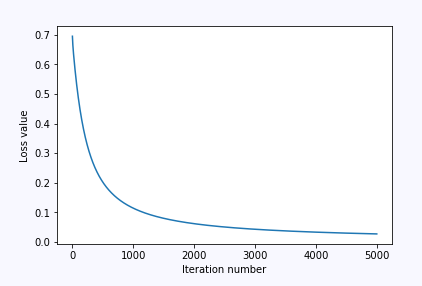
训练测试一下,并且可视化跟踪的损失loss
import matplotlib.pyplot as plt
y = y.reshape((-1,1))
#add the x0=1
one = np.ones((X.shape[0],1))
X_train = np.hstack((one,X))
classify = logistic()
loss = classify.train(X_train,y)
print classify.W
plt.plot(loss)
plt.xlabel('Iteration number')
plt.ylabel('Loss value')
plt.show() |
最后可视化“决策边界”
label = np.array(y)
index_0 = np.where(label==0)
plt.scatter(X[index_0,0],X[index_0,1], marker='x',color
= 'b',label = '0',s = 15)
index_1 =np.where(label==1)
plt.scatter(X[index_1,0],X[index_1,1], marker='o',color
= 'r',label = '1',s = 15)
#show the decision boundary
x1 = np.arange(4,7.5,0.5)
x2 = (- classify.W[0] - classify.W[1]*x1) / classify.W[2]
plt.plot(x1,x2,color = 'black')
plt.xlabel('X1')
plt.ylabel('X2')
plt.legend(loc = 'upper left')
plt.show()
|
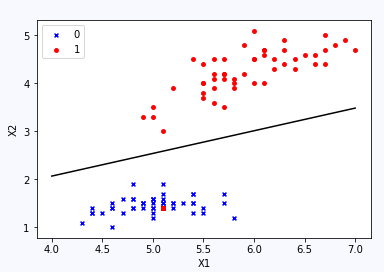
ps:可以看出,最后学习得到的决策边界(分类边界)成功的隔开了两个类别。当然,分类问题还有多分类问题(一对多),还有就是对于非线性分类问题,详情请参见分享的资料。 |